Speech Recognition System
Summary
Research and development of a speech recognition system in Matlab using characteristics of the glottal pulse. Design a complete speech recognition system catching every glottal pulse and separating it from background noise, calculating the average of all stimuli and analyzing in the temporal domain and spectral domain. With the obtained results, determine the optimal threshold so as to ultimately obtain a program with an effectiveness of 80%
Preprocessing
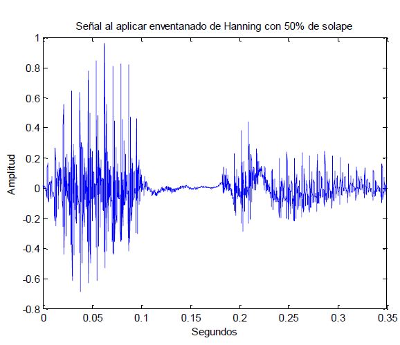
First of all, we record the word “cuatro” (four in Spanish) why this word? Because when we are making voice, the only sound that matter for speech recognition are the vowels because the consonants only introduce white noise, and that is useless for us. As soon as we have the word “cuatro” recorded, we normalize it and print it to see how it looks:
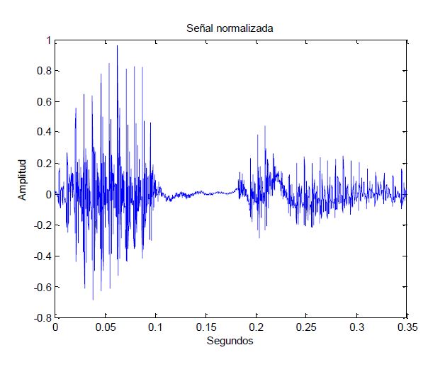
As we can see, the first part represents the sound “ua” and the second part the “o”, the rest will be white noise as we will show afterwards using the spectrogram, but as the group imagine dragons said, “First things first”.
After this, we will apply a Hanning window every 160 samples with 50% overlapping for research purposes on the voice, here we will see how it looks after applying to one window:
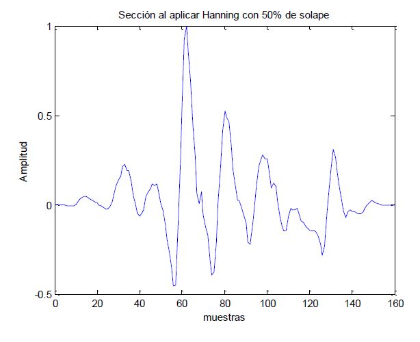
Looks good right? So now we will apply the same window to all our record, having as a result:
Now that we have our example normalized and windowed we will need to apply LPC (Linear Predictive Coding) to our sample using exactly 12 coefficients (less is not accurate and more is too much computational cost). Why do we do this? Well, let me first show you how it looks and explain it to you what does this do:
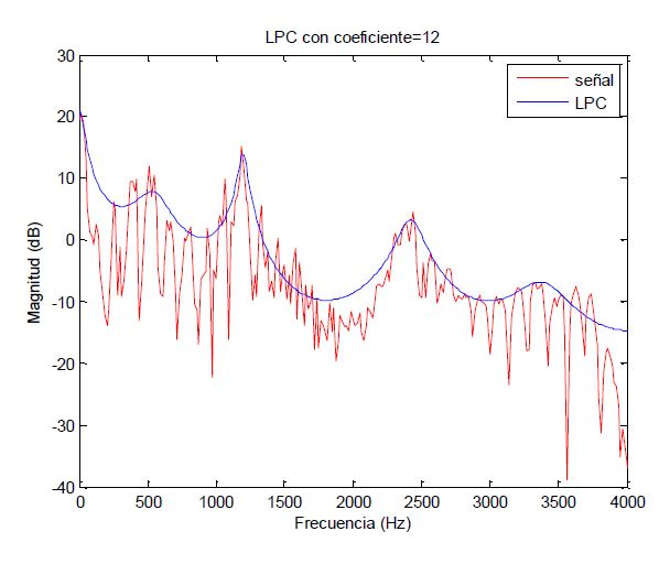
As we can see, the LPC with 12 coefficients is really accurate approaching to our voice record, and now the question that all is waiting for… Drums playing in the background we do this because after some math that I will not go deeper, if we apply the inverse of this linear predictive approach, we will obtain the residue of the voice, and we will be working on that.
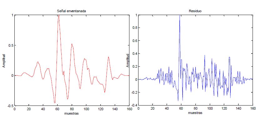
Here probably you can not see a big difference or why we should be working with the residue, but wait for the next image and you will understand better.
This will be really useful because as we can see, it makes our maximums more pronounced and the noise it is really easy to detect (in the middle, representing the “tr” sound). Now that we have the signal that we wanted to work with, let’s have a small break, sipping some tea and let us continue.
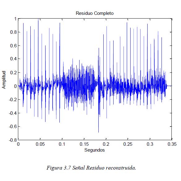
But wait! As we can see, or signal has a bit of curvature, it seems like a roller coaster.
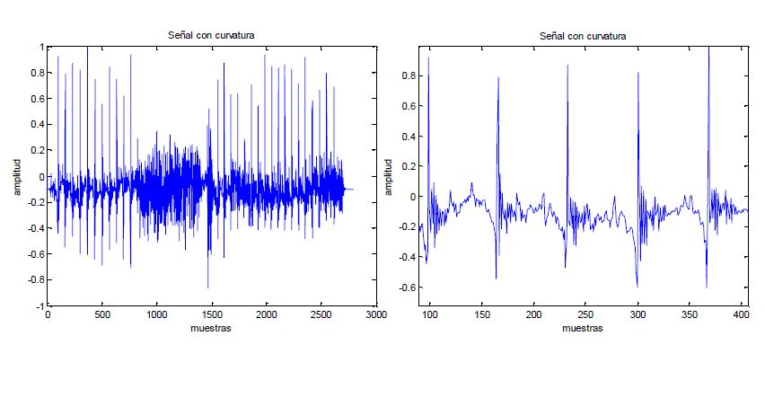
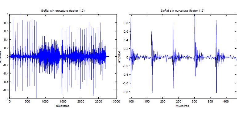
Do not worry, I will solve this for those persons who hate roller coasters applying an LMS algorithm (Least-Mean Square) with 1.2 as the factor, having as a result the next image.
And as I promised before, if we make the spectrogram of the original voice, we will get this:
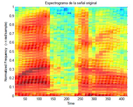
As we can imagine, those red labels are where the vowels are located.
LET’S GET HANDS INTO THE PROJECT
If you arrived here it is a miracle, I do not like the spoilers, but sorry, I will do it… At the end I will get an 80% of effectiveness.
Now, talking seriously, after getting the signal as we wanted, we will apply a threshold to delete the white noise and also to take different maximums + certain samples (140 in total) to get different pieces of the voice, from now on we will call them pulses. After getting all those pulses and introduce them in a matrix, we make the average of all of them and we get this:
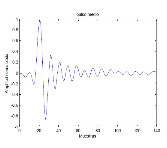
With this pulse, we will work with two things, first we will gather all the positions where a maximum or a minimum is located in one vector, and we will gather the amplitude or those maximum or minimum in another vector, from now on they will be called vector “A” for the localization, and “B” for the amplitude.
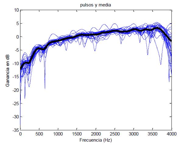
But this is not all, now we will convert from the temporary scope to the spectral field (Or frequency field if that makes you understand it better) getting the following image highlighting in black the average of all the different pulses, and after being saved in the vector “C”
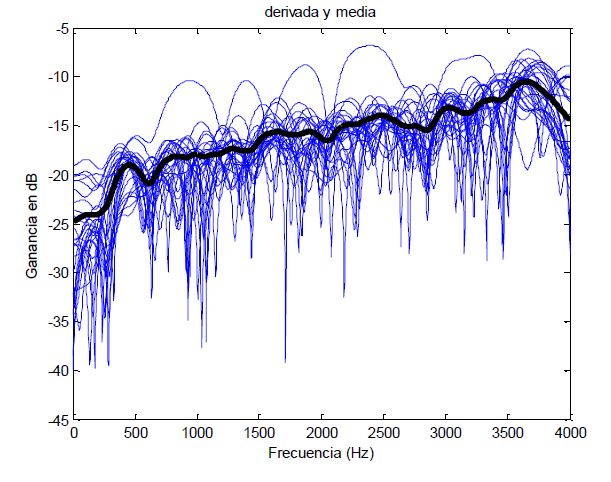
No, this is not the Jackson 5 song “ABC” because as Maluma says, “Felices los 4”, so we will add another vector called “D” that will be the difference (or Derivatives if you prefer it) getting the following image:
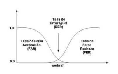
False Acceptance and False Rejection
After seeing all this data you will need to trust me that the vector “A” (the one with the position of the maximums and minimums) will not be really useful, so from now on we will be working with the other 3. After applying some statistics, and knowing that there are two different cases: false acceptance and false rejection, we will need to apply a confidence threshold that will be where those two collide.
So now we will see in our case in the different vectors “B” “C” “D”
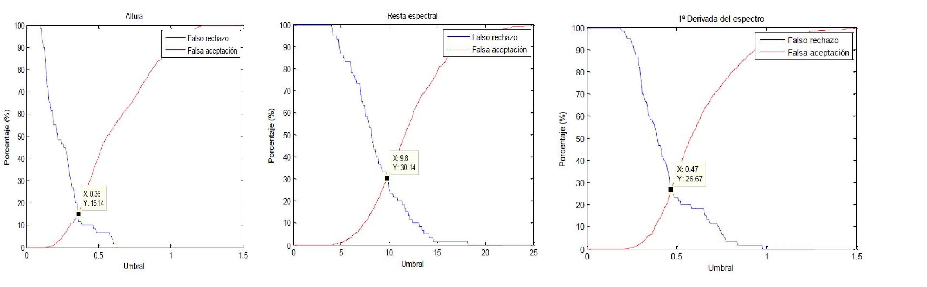
And after applying those thresholds and seeing the results, with the vector “B” (the one with the value of the appliance of the maximums and minimums) we will get an 84% of effectiveness, so I guess we have a winner.
Of course, if you want to know more about the project do not hesitate to contact me, and you will be able to download it with the following button:
Note- Sorry, my thesis is in Spanish so make yourself a Mojito/Sangria and enjoy the moment. Cheers.